
Data manipulation with PivotTables
You can use PivotTables to manipulate and filter the data in your Asset Tracking XML Data Dump.
The option to download the XML or SQL Data Dump is only available for contracted customers.
PivotTables are one option to manipulate the data but you can choose other options, such as a Microsoft Excel Power Query.
PivotTable example
In this basic example, you will see how to create a 'software report' from an Asset Tracking XML Data Dump using Microsoft Excel.
Some features may not be available in Microsoft Excel Online due to its reduced functionality. See Microsoft's article Create a PivotTable to analyze worksheet data for details and usage of PivotTables in Excel.
Download the XML file
- Use Export a hardware and software data dump to gather data for all or a specific client.
- Save the file when prompted.
Open the XML file in Excel
- In Excel, select Open, browse to and select the saved data dump file.
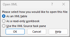
- If prompted, choose As an XML table from the Open XML dialog.
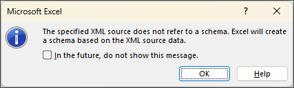
- Select OK in the schema advisory dialog if it displays.
Default file name: <saved-date>_asset_tracking_data_dump.xml.
Insert PivotTable
- After the data loads in Excel, highlight a range of data to include. If you do not highlight data, the whole table is selected.
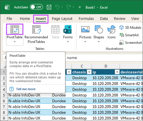
- Go to Insert and select PivotTable from the Tables section .
- In the Create PivotTable dialog, review the Select a table or range settings and Choose where you want the PivotTable to be placed, in a new or existing worksheet and select OK to apply.
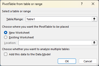
In this example, the full table was chosen, and the PivotTable created as a New Worksheet.
Populate the PivotTable
Each column of the Asset Tracking XML Data Dump contains a heading that is displayed under the PivotTable Fields section.
You can edit column headings to a more meaningful name by editing them before or after the PivotTable is created.
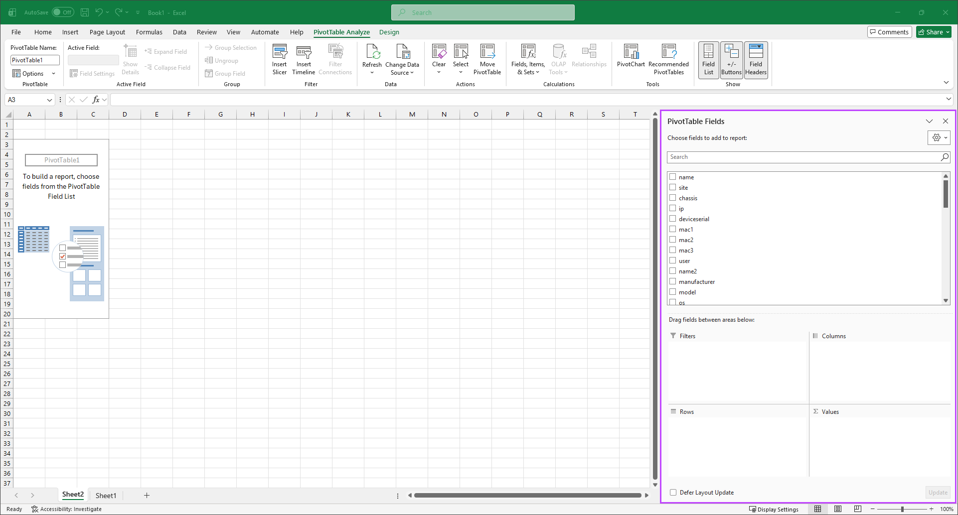
- Populate the PivotTable by selecting the required fields from the PivotTable Fields section.
- Right-click the field name to open the selection context menu, or
- Add it as a Row label and then drag and drop it to the required area.
- Re-order the list of included fields as needed to create your PivotTable.
When you select a field, it will automatically be added as a Row. To set it as a Filter, Column or Value, either
When adding the required fields, it is useful to refer back to the source spreadsheet for details on the information each column contains.
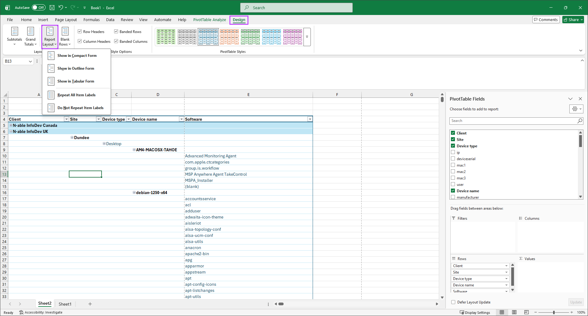
Refine the PivotTable
You can refine the populated PivotTable using the PivotTable Options, accessed by right-clicking in the table. These options allow you to set the Layout & Format, Totals & Filters, Display elements, Printing options, Data storage & retention, and Alt Text definitions.
You can also edit each PivotTable field header by right-clicking it.
For our 'software report' example we chose the following fields (and renamed them);
name(Client)site(Site)chassis(Device type)name2(Device name)name6(Software)
You can control the look using Excel's Design tools. In the below screenshot, we altered the layout using the Report Layout options and styles.
When you are finished configuring your report, you can save and print it for presentation to your customer.